Compare Two Excel Ranges
Got any Excel/VBA Questions? Free Excel Help
When you have two large tables of data in an Excel Workbook you may need to compare the tables to try and spot the differences. Below we will look at two very easy ways this can be done which will save you hours of manual work.
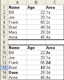
For both examples I will use the two ranges shown in the screen shot below. Note that I have bolded the cells in the second table that are not the same as their counterpart in the first table for easier viewing.
Method 1 - Using True or False
The first method involves entering a simple formula in another identically sized and shaped range. The best part of this method is that we can add the formulas in one step without having to copy and paste.
- Using The Above Ranges To Compare Select The Range E1:G7 Starting From Cell E1. This Ensures That E1 Is The Active Cell In The Selection.
- With This Range Selected Click In The Formula Bar And Type In: =A1=A9
- Now Enter This Formula By Pushing Ctrl+Enter At The Same Time
You should now see the range E1:G7 filled with True (the same) and False (not the same).
Method 2 - Using Conditional Formatting
The second method is often the preferred way as it is easier to make any needed changes once the comparison has been done.
- Using The Above Ranges To Compare, Select The Range A1:C7 Stating From Cell A1. This Ensures That A1 Is The Active Cell In The Selection.
- With This Range Selected, Go To Format>Conditional Formatting
- Select Formula Is And Then Type The Formula =NOT(A1=A9)
- Click The Format Button And Choose The Format To Mark Differences With. I Have Used An Orange Background.
Now simply click OK and all your differences will be formatted according to the format you have chosen. When or if you make any changes the cells format will automatically revert back to normal if the cell content is the same as the cell in the other table.
See also: Index to Excel VBA Code and Index to Excel Freebies and Lesson 1 - Excel Fundamentals and Index to how to… providing a range of solutions and Index to new resources and reference sheets
See also:
| Calculate a Person's Age in Excel |
| Converting, Text Case & Importing for Excel |
| Lookup Value & Return Corresponding Result |
| Split Chart Graphic Picture Into Variable Width Sections |
Microsoft ® and Microsoft Excel ® are registered trademarks of Microsoft Corporation. OzGrid is in no way associated with Microsoft.
Click here to visit our Free 24/7 Excel/VBA Help Forum where there are thousands of posts you can get information from, or you can join the Forum and post your own questions.


