 |
Software Search, Categories and Specials | Similar Products Monte Carlo Financial Modeling Multiple Target Goal Seek What-If Analysis Manager Excel Model Builder Finance & Statistics Model Set |
 |
Software Search, Categories and Specials | Similar Products Monte Carlo Financial Modeling Multiple Target Goal Seek What-If Analysis Manager Excel Model Builder Finance & Statistics Model Set |
| Buy Today (below) and send us your order ID and claim over $70.00 worth of FREE software |
|---|
This guide describes how to convert a static Excel spreadsheet model into a Monte Carlo simulation, and the kind of information you can learn from the simulation.
The examples in this guide use the Monte Carlo add-in; if you don't have the add-in already, you can download a free trial version from our download page .
Investment Portfolio Model
Download the spreadsheet used in this example Zip File or, Excel File
A typical investment portfolio model includes an opening balance, projections for returns and costs over several years, and a closing balance at some time in the future. A simple spreadsheet model might look like this:
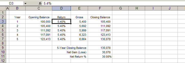
In figure A, the model is based on a fixed period (annual) return of 5.4%. Over the course of 5 years, this results in a return of 30.08%.
While the 5.4% is an expected return, we know that actual returns can vary greatly. The first step in building the Monte Carlo model is replacing these fixed returns with randomly distributed values, to better approximate the real world.
� Step 1: Adding Random Data
In the Monte Carlo model, instead of a fixed 5.4% return, we anticipate that the return will be normally distributed with a mean (average) of 5.4% and a standard deviation of 7.3%. For each return cell in the spreadsheet (column D), we use the random function NormalValue:
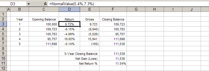
In figure B, the return in each period has been changed from a fixed 5.4% to a randomly distributed return, using the function seen in the function bar. The returns in each period are randomly generated. In Excel, if you recalculate the spreadsheet at this step (press Ctrl+Alt+F9), you will see each return change. The total return (cell F11) can also differ significantly from the original value (30.08%).
Randomly-distributed returns seem like a better approximation of the real world, but taking a single random return isn't useful. The key to using Monte Carlo simulation is to take many random values and analyze the overall results.
� Step 2: Running a Monte Carlo Simulation
A Monte Carlo simulation calculates the same model many many times, and generates useful information from the overall results. To run a Monte Carlo simulation, select "Monte Carlo" -> "Run Monte Carlo Simulation..." from the menu. When the simulation dialog is open, click "Start " to run a simulation. You'll see the random values in the model changing again and again while the simulation runs.
The Add-in includes a number of functions to analyze the results of a Monte Carlo simulation. To Start , we'll look at the average results of the simulation using the SimulationAverage function.
Note: the first time you enter these functions in a spreadsheet, you'll see an #N/A error. This is because the simulation hasn't collected data for the cell yet. Once you run a simulation, this error will go away.
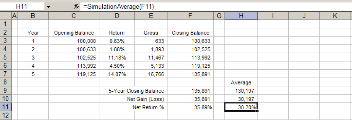
In Figure C, we've added average simulation results in column H using the function seen in the function bar. In this example, cell H11 calculates the average value of cell F11 over all the trials, or iterations, of the Monte Carlo simulation. To see how it works, run a Monte Carlo simulation using the menu item "Monte Carlo" -> "Run Monte Carlo Simulation...". You'll see the value of F11 change at each trial, but the value in H11 slowly Start s to settle down at the average value.
When you run a Monte Carlo simulation, at each iteration new random values are placed in column D and the spreadsheet is recalculated. This results in a different value in cell F11. The Monte Carlo simulation runs hundreds or thousands of times, and at each iteration the Add-in stores and remembers the value of cell F11. Once the simulation is complete, the average value can be calculated from this set of stored values.
You'll see that the average value, returned in cell H11, is very close to the original fixed value of 30.08% (see cell F11 in Figure A). This is as expected, because the random data we're using for returns has an average of 5.4%, which was the fixed value in the original model.
� Step 3: Analyzing Data
As noted above, the average return given by the Monte Carlo simulation is close to the original, fixed model. If that were the only thing we could learn from the simulation, it wouldn't have much use. However, we can get much more useful information from the Monte Carlo simulation by looking at ranges and percentiles.
To begin with, we can look at the minimum and maximum values identified during the simulation using the SimulationMin and SimulationMax functions:
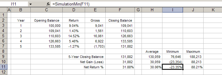
In Figure D, cell I11 contains the minimum value of cell F11 seen during the simulation. This is significantly worse then the average, and represents the risk contained in the portfolio model. This means that there is some possibility that this portfolio, over 5 years, will wind up with a net loss of 23%.
Looking at the absolute miniumum and maximum values tends to overstate the outliers, or edges, of the possible outcomes of the portfolio model. We can also look at percentile probabilities, using the SimulationPercentile function:
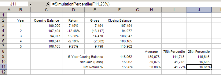
In Figure E, cell J11 contains the SimulationPercentile function as seen in the function bar. To understand what the percentiles mean, imagine that we take every result seen in cell F11 over the Monte Carlo simulation, and place them in order (lowest to highest). The first value would be the minimum, as seen above; no values in the results are lower than the minimum value. The last value would be the maximum; 100% of the values in the results are equal to, or lower than, the last value. Therefore the maximum value is the 100th Percentile.
The 25th Percentile, then, represents a value that is equal to or higher than 25% of the results seen during the simulation. Another way to say it is, there is a 25% chance that any value in the simulation will be lower to or equal to this amount; and at the same time, there is a 75% chance that any value in the simulation will be higher than or equal to this amount.
In Figure E, cell J11 shows the 25th Percentile result for cell F11. This tells us that, over the simulation, 75% of the time the value of F11 is higher than or equal to 16.61%. Or, there is a 75% chance that our model will have a total return of 16.61% or higher.
By changing the percentile values, we can determine the expected return of the portfolio with different probabilities. This kind of analysis can be useful in determining the real levels of risk associated with an investment portfolio.
� Step 4: Determining Confidence Levels
Instead of finding the expected return at different percentiles, we can turn the analysis around and find the probability of reaching a particular target return with the SimulationInterval function:
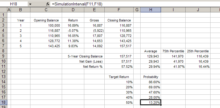
This analysis answers the question, what is the likelihood, over all trials of the simulation, that the model will return at least 50%? In Figure F, this probability is 13.20%; that is, there is a 13.20% probability the model will result in a return of 50% or more. This kind of analysis can be useful in determining confidence levels. For example, in evaluating alternative investments, we can compare the probabilities of reaching certain minimum returns. Or we can understand the probability of loss associated with an investment by finding the likelihood that it will return 0%.
� Conclusion
The above discussion describes converting a simple fixed portfolio model into a Monte Carlo simulation, and the kinds of analysis that can be done with a Monte Carlo simulation. This is a very simple example; many different analysis functions are available, and there are many different ways to generate random data in a model. See the Help Manual (available in Excel or from the Start Menu) for more information about the various functions.
Of course any analysis is only as good as the model and the data that are entered. This model is very simple in that it ignores investment costs and inflation. The model is also very sensitive to the mean and standard deviation of our expected return.
Nevertheless, it's evident from the analysis that the simple fixed model hides much of the risk associated with the portfolio. By using a Monte Carlo simulation, and with some basic analysis of the results, we have a lot more detailed information about the possible outcomes of this portfolio.
 $129.95
Special! Free Choice of Complete Excel Training Course or Excel Add-ins Collection on all purchases totaling over $70.00. ALL purchases totaling over $150.00 gets you BOTH! Purchases MUST be made via this site. Send payment proof to [email protected] 31 days after purchase date.
Microsoft � and Microsoft Excel � are registered trademarks of Microsoft Corporation. OzGrid is in no way associated with Microsoft
SPECIALS!
Convert Excel Spreadsheets To Webpages | Trading In Excel | Construction Estimators | Finance Templates & Add-ins Bundle | Code-VBA | Smart-VBA | Print-VBA | Excel Data Manipulation & Analysis | Convert MS Office Applications To...... | Analyzer Excel | Downloader Excel
| MSSQL Migration
Toolkit |
Monte Carlo Add-in |
Excel
Costing Templates